Climate sensitivity, sea level and atmospheric carbon dioxide Authors
AbstractCenozoic temperature, sea level and CO2 covariations provide insights into climate sensitivity to external forcings and sea-level sensitivity to climate change. Climate sensitivity depends on the initial climate state, but potentially can be accurately inferred from precise palaeoclimate data. Pleistocene climate oscillations yield a fast-feedback climate sensitivity of 3±1°C for a 4 W m−2 CO2 forcing if Holocene warming relative to the Last Glacial Maximum (LGM) is used as calibration, but the error (uncertainty) is substantial and partly subjective because of poorly defined LGM global temperature and possible human influences in the Holocene. Glacial-to-interglacial climate change leading to the prior (Eemian) interglacial is less ambiguous and implies a sensitivity in the upper part of the above range, i.e. 3–4°C for a 4 W m−2 CO2 forcing. Slow feedbacks, especially change of ice sheet size and atmospheric CO2, amplify the total Earth system sensitivity by an amount that depends on the time scale considered. Ice sheet response time is poorly defined, but we show that the slow response and hysteresis in prevailing ice sheet models are exaggerated. We use a global model, simplified to essential processes, to investigate state dependence of climate sensitivity, finding an increased sensitivity towards warmer climates, as low cloud cover is diminished and increased water vapour elevates the tropopause. Burning all fossil fuels, we conclude, would make most of the planet uninhabitable by humans, thus calling into question strategies that emphasize adaptation to climate change. 1. IntroductionHumanity is now the dominant force driving changes in the Earth’s atmospheric composition and climate [1]. The largest climate forcing today, i.e. the greatest imposed perturbation of the planet’s energy balance [1,2], is the human-made increase in atmospheric greenhouse gases (GHGs), especially CO2 from the burning of fossil fuels. Earth’s response to climate forcings is slowed by the inertia of the global ocean and the great ice sheets on Greenland and Antarctica, which require centuries, millennia or longer to approach their full response to a climate forcing. This long response time makes the task of avoiding dangerous human alteration of climate particularly difficult, because the human-made climate forcing is being imposed rapidly, with most of the current forcing having been added in just the past several decades. Thus, observed climate changes are only a partial response to the current climate forcing, with further response still ‘in the pipeline’ [3]. Climate models, numerical climate simulations, provide one way to estimate the climate response to forcings, but it is difficult to include realistically all real-world processes. Earth’s palaeoclimate history allows empirical assessment of climate sensitivity, but the data have large uncertainties. These approaches are usually not fully independent, and the most realistic eventual assessments will be ones combining their greatest strengths. We use the rich climate history of the Cenozoic era in the oxygen isotope record of ocean sediments to explore the relation of climate change with sea level and atmospheric CO2, inferring climate sensitivity empirically. We use isotope data from Zachos et al. [4], which are improved over data used in our earlier study [5], and we improve our prescription for separating the effects of deep ocean temperature and ice volume in the oxygen isotope record as well as our prescription for relating deep ocean temperature to surface air temperature. Finally, we use an efficient climate model to expand our estimated climate sensitivities beyond the Cenozoic climate range to snowball Earth and runaway greenhouse conditions. 2. Overview of Cenozoic climate and our analysis approachThe Cenozoic era, the past 65.5 million years (Myr), provides a valuable perspective on climate [5,6] and sea-level change [7], and Cenozoic data help clarify our analysis approach. The principal dataset we use is the temporal variation of the oxygen isotope ratio (δ18O relative to δ16O; figure 1a right-hand scale) in the shells of deep-ocean-dwelling microscopic shelled animals (foraminifera) in a near-global compilation of ocean sediment cores [4]. δ18O yields an estimate of the deep ocean temperature (figure 1b), as discussed in §3. Note that coarse temporal resolution of δ18O data in the intervals 7–17, 35–42 and 44–65 Myr reduces the apparent amplitude of glacial–interglacial climate fluctuations (see electronic supplementary material, figure S1). We use additional proxy measures of climate change to supplement the δ18O data in our quantitative analyses. 
View larger version:
Figure 1.(a) Global deep ocean δ18O from Zachos et al. [4] and (b) estimated deep ocean temperature based on the prescription in our present paper. Black data points are five-point running means of the original temporal resolution; red and blue curves have a 500 kyr resolution. Coarse temporal sampling reduces the amplitude of glacial–interglacial oscillations in the intervals 7–17, 35–42 and 44–65 Myr BP.
Carbon dioxide is involved in climate change throughout the Cenozoic era, both as a climate forcing and as a climate feedback. Long-term Cenozoic temperature trends, the warming up to about 50 Myr before present (BP) and subsequent long-term cooling, are likely to be, at least in large part, a result of the changing natural source of atmospheric CO2, which is volcanic emissions that occur mainly at continental margins due to plate tectonics (popularly ‘continental drift’); tectonic activity also affects the weathering sink for CO2 by exposing fresh rock. The CO2 tectonic source grew from 60 to 50 Myr BP as India subducted carbonate-rich ocean crust while moving through the present Indian Ocean prior to its collision with Asia about 50 Myr BP [8], causing atmospheric CO2 to reach levels of the order of 1000 ppm at 50 Myr BP [9]. Since then, atmospheric CO2 declined as the Indian and Atlantic Oceans have been major depocentres for carbonate and organic sediments while subduction of carbonate-rich crust has been limited mainly to small regions near Indonesia and Central America [10], thus allowing CO2 to decline to levels as low as 170 ppm during recent glacial periods [11]. A climate forcing due to a CO2 change from 1000 to 170 ppm is more than 10 W m−2, which compares with forcings of the order of 1 W m−2 for competing climate forcings during the Cenozoic era [5], specifically long-term change of solar irradiance and change of planetary albedo (reflectance) owing to the overall minor displacement of continents in that era. Superimposed on the long-term trends are occasional global warming spikes, ‘hyperthermals’, most prominently the Palaeocene–Eocene Thermal Maximum (PETM) at approximately 56 Myr BP [12] and the Mid-Eocene Climatic Optimum at approximately 42 Myr BP [13], coincident with large temporary increases of atmospheric CO2. The most studied hyperthermal, the PETM, caused global warming of at least 5°C coincident with injection of a likely 4000–7000 Gt of isotopically light carbon into the atmosphere and ocean [14]. The size of the carbon injection is estimated from changes in the stable carbon isotope ratio 13C/12C in sediments and from ocean acidification implied by changes in the ocean depth below which carbonate dissolution occurred. The potential carbon source for hyperthermal warming that received most initial attention was methane hydrates on continental shelves, which could be destabilized by sea floor warming [15]. Alternative sources include release of carbon from Antarctic permafrost and peat [16]. Regardless of the carbon source(s), it has been shown that the hyperthermals were astronomically paced, spurred by coincident maxima in the Earth’s orbit eccentricity and spin axis tilt [17], which increased high-latitude insolation and warming. The PETM was followed by successively weaker astronomically paced hyperthermals, suggesting that the carbon source(s) partially recharged in the interim [18]. A high temporal resolution sediment core from the New Jersey continental shelf [19] reveals that PETM warming in at least that region began about 3000 years prior to a massive release of isotopically light carbon. This lag and climate simulations [20] that produce large warming at intermediate ocean depths in response to initial surface warming are consistent with the concept of a methane hydrate role in hyperthermal events. The hyperthermals confirm understanding about the long recovery time of the Earth’s carbon cycle [21] and reveal the potential for threshold or ‘tipping point’ behaviour with large amplifying climate feedback in response to warming [22]. One implication is that if humans burn most of the fossil fuels, thus injecting into the atmosphere an amount of CO2 at least comparable to that injected during the PETM, the CO2 would stay in the surface carbon reservoirs (atmosphere, ocean, soil, biosphere) for tens of thousands of years, long enough for the atmosphere, ocean and ice sheets to fully respond to the changed atmospheric composition. In addition, there is the potential that global warming from fossil fuel CO2 could spur release of CH4 and CO2 from methane hydrates or permafrost. Carbon release during the hyperthermals required several thousand years, but that long injection time may have been a function of the pace of the astronomical forcing, which is much slower than the pace of fossil fuel burning. The Cenozoic record also reveals the amplification of climate change that occurs with growth or decay of ice sheets, as is apparent at about 34 Myr BP when the Earth became cool enough for large-scale glaciation of Antarctica and in the most recent 3–5 Myr with the growth of Northern Hemisphere ice sheets. Global climate fluctuated in the 20 Myr following Antarctic glaciation with warmth during the Mid-Miocene Climatic Optimum (MMCO, 15 Myr BP) possibly comparable to that at 34 Myr BP, as, for example, Germany became warm enough to harbour snakes and crocodiles that require an annual temperature of about 20°C or higher and a winter temperature more than 10°C [23]. Antarctic vegetation in the MMCO implies a summer temperature of approximately 11°C warmer than today [24] and annual sea surface temperatures ranging from 0°C to 11.5°C [25]. Superimposed on the long-term trends, in addition to occasional hyperthermals, are continual high-frequency temperature oscillations, which are apparent in figure 1 after 34 Myr BP, when the Earth became cold enough for a large ice sheet to form on Antarctica, and are still more prominent during ice sheet growth in the Northern Hemisphere. These climate oscillations have dominant periodicities, ranging from about 20 to 400 kyr, that coincide with variations in the Earth’s orbital elements [26], specifically the tilt of the Earth’s spin axis, the eccentricity of the orbit and the time of year when the Earth is closest to the Sun. The slowly changing orbit and tilt of the spin axis affect the seasonal distribution of insolation [27], and thus the growth and decay of ice sheets, as proposed by Milankovitch [28]. Atmospheric CO2, CH4 and N2O have varied almost synchronously with global temperature during the past 800 000 years for which precise data are available from ice cores, the GHGs providing an amplifying feedback that magnifies the climate change instigated by orbit perturbations [29–31]. Ocean and atmosphere dynamical effects have been suggested as possible causes of some climate change within the Cenozoic era; for example, topographical effects of mountain building [32], closing of the Panama Seaway [33] or opening of the Drake Passage [34]. Climate modelling studies with orographic changes confirm significant effects on monsoons and on Eurasian temperature [35]. Modelling studies indicate that closing of the Panama Seaway results in a more intense Atlantic thermohaline circulation, but only small effects on Northern Hemisphere ice sheets [36]. Opening of the Drake Passage surely affected ocean circulation around Antarctica, but efforts to find a significant effect on global temperature have relied on speculation about possible effects on atmospheric CO2 [37]. Overall, there is no strong evidence that dynamical effects are a major direct contributor to Cenozoic global temperature change. We hypothesize that the global climate variations of the Cenozoic (figure 1) can be understood and analysed via slow temporal changes in Earth’s energy balance, which is a function of solar irradiance, atmospheric composition (specifically long-lived GHGs) and planetary surface albedo. Using measured amounts of GHGs during the past 800 000 years of glacial–interglacial climate oscillations and surface albedo inferred from sea-level data, we show that a single empirical ‘fast-feedback’ climate sensitivity can account well for the global temperature change over that range of climate states. It is certain that over a large climate range climate sensitivity must become a strong function of the climate state, and thus we use a simplified climate model to investigate the dependence of climate sensitivity on the climate state. Finally, we use our estimated state-dependent climate sensitivity to infer Cenozoic CO2 change and compare this with proxy CO2 data, focusing on the Eocene climatic optimum, the Oligocene glaciation, the Miocene optimum and the Pliocene. 3. Deep ocean temperature and sea level in the Cenozoic eraThe δ18O stable isotope ratio was the first palaeothermometer, proposed by Urey [38] and developed especially by Emiliani [39]. There are now several alternative proxy measures of ancient climate change, but the δ18O data (figure 1a) of Zachos et al. [4], a conglomerate of the global ocean sediment cores, is well suited for our purpose as it covers the Cenozoic era with good temporal resolution. There are large, even dominant, non-climatic causes of δ18O changes over hundreds of millions of years [40], but non-climatic change may be small in the past few hundred million years [41] and is generally neglected in Cenozoic climate studies. The principal difficulty in using the δ18O record to estimate global deep ocean temperature, in the absence of non-climatic change, is that δ18O is affected by the global ice mass as well as the deep ocean temperature. We make a simple estimate of global sea-level change for the Cenozoic era using the near-global δ18O compilation of Zachos et al. [4]. More elaborate and accurate approaches, including use of models, will surely be devised, but comparison of our result with other approaches is instructive regarding basic issues such as the vulnerability of today’s ice sheets to near-term global warming and the magnitude of hysteresis effects in ice sheet growth and decay. During the Early Cenozoic, between 65.5 and 35 Myr BP, the Earth was so warm that there was little ice on the planet and the deep ocean temperature is approximated by [6] This approximation can easily be made more realistic. Although ice volume and deep ocean temperature changes contributed comparable amounts to δ18O change on average over the full range from 35 Myr to 20 kyr BP, the temperature change portion of the δ18O change must decrease as the deep ocean temperature approaches the freezing point [43]. The rapid increase in δ18O in the past few million years was associated with the appearance of Northern Hemisphere ice sheets, symbolized by the dark blue bar in figure 1a. The sea-level change between the LGM and Holocene was approximately 120 m [44,45]. Thus, two-thirds of the 180 m sea-level change between the ice-free planet and the LGM occurred with formation of Northern Hemisphere ice (and probably some increased volume of Antarctic ice). Thus, rather than taking the 180 m sea-level change between the nearly ice-free planet of 34 Myr BP and the LGM as being linear over the entire range (with 90 m for δ18O<3.25 and 90 m for δ18O>3.25), it is more realistic to assign 60 m of sea-level change to δ18O 1.75–3.25 and 120 m to δ18O>3.25. The total deep ocean temperature change of 6°C for the change of δ18O from 1.75 to 4.75 is then divided two-thirds (4°C) for the δ18O range 1.75–3.25 and 2°C for the δ18O range 3.25–4.75. Algebraically, Sea level from equations (3.3) and (3.4) is shown by the blue curves in figure 2, including comparison (figure 2c) with the Late Pleistocene sea-level record of Rohling et al. [47], which is based on analysis of Red Sea sediments, and comparison (figure 2b) with the sea-level chronology of de Boer et al. [46], which is based on ice sheet modelling with the δ18O data of Zachos et al. [4] as a principal input driving the ice sheet model. Comparison of our result with that of de Boer et al. [46] for the other periods of figure 2 is included in the electronic supplementary material, where we also make available our numerical data. Deep ocean temperature from equations (3.5) and (3.6) is shown for the Pliocene and Pleistocene in figure 3 and for the entire Cenozoic era in figure 1. 
View larger version:

View larger version:
Figure 3.Deep ocean temperature in (a) the Pliocene and Pleistocene and (b) the last 800 000 years. High-frequency variations (black) are five-point running means of the original data [4], whereas the blue curve has a 500 kyr resolution. The deep ocean temperature for the entire Cenozoic era is in figure 1b.
Differences between our inferred sea-level chronology and that from the ice sheet model [46] are relevant to the assessment of the potential danger to humanity from future sea-level rise. Our estimated sea levels have reached +5 to 10 m above the present sea level during recent interglacial periods that were barely warmer than the Holocene, whereas the ice sheet model yields maxima at most approximately 1 m above the current sea level. We find the Pliocene sea level varying between about +20 m and −50 m, with the Early Pliocene averaging about +15 m; the ice sheet model has a less variable sea level with the Early Pliocene averaging about +8 m. A 15 m sea-level rise implies that the East Antarctic ice sheet as well as West Antarctica and Greenland ice were unstable at a global temperature no higher than those projected to occur this century [1,48]. How can we interpret these differences, and what is the merit of our simple δ18O scaling? Ice sheet models constrained by multiple observations may eventually provide our best estimate of sea-level change, but as yet models are primitive. Hansen [49,50] argues that real ice sheets are more responsive to climate change than is found in most ice sheet models. Our simple scaling approximation implicitly assumes that ice sheets are sufficiently responsive to climate change that hysteresis is not a dominant effect; in other words, ice volume on millennial time scales is a function of temperature and does not depend much on whether the Earth is in a warming or cooling phase. Thus, our simple transparent calculation may provide a useful comparison with geological data for sea-level change and with results of ice sheet models. We cannot a priori define accurately the error in our sea-level estimates, but we can compare with geological data in specific cases as a check on reasonableness. Our results (figure 2) yield two instances in the past million years when sea levels have reached heights well above the current sea level: +9.8 m in the Eemian (approx. 120 kyr BP, also known as Marine Isotope Stage 5e or MIS-5e) and +7.1 m in the Holsteinian (approx. 400 kyr BP, also known as MIS-11). Indeed, these are the two interglacial periods in the Late Pleistocene that traditional geological methods identify as probably having a sea level exceeding that in the Holocene. Geological evidence, mainly coral reefs on tectonically stable coasts, was described in the review of Overpeck et al. [51] as favouring an Eemian maximum of +4 to more than 6 m. Rohling et al. [52] cite many studies concluding that the mean sea level was 4–6 m above the current sea level during the warmest portion of the Eemian, 123–119 kyr BP; note that several of these studies suggest Eemian sea-level fluctuations up to +10 m, and provide the first continuous sea-level data supporting rapid Eemian sea-level fluctuations. Kopp et al. [53] made a statistical analysis of data from a large number of sites, concluding that there was a 95% probability that the Eemian sea level reached at least +6.6 m with a 67% probability that it exceeded 8 m. The Holsteinian sea level is more difficult to reconstruct from geological data because of its age, and there has been a long-standing controversy concerning a substantial body of geological shoreline evidence for a +20 m Late Holsteinian sea level that Hearty and co-workers have found on numerous sites [54,55] (numerous pros and cons are contained in the references provided in our present paragraph). Rohling et al. [56] note that their temporally continuous Red Sea record ‘strongly supports the MIS-11 sea level review of Bowen [57], which also places MIS-11 sea level within uncertainties at the present-day level’. This issue is important because both ice core data [29] and ocean sediment core data (see below) indicate that the Holsteinian period was only moderately warmer than the Holocene with similar Earth orbital parameters. We suggest that the resolution of this issue is consistent with our estimate of the approximately +7 m Holsteinian global sea level, and is provided by Raymo & Mitrovica [58], who pointed out the need to make a glacial isostatic adjustment (GIA) correction for post-glacial crustal subsidence at the places where Hearty and others deduced local sea-level change. The uncertainties in GIA modelling led Raymo & Mitrovica [58] to conclude that the peak Holsteinian global sea level was in the range of +6 to 13 m relative to the present. Thus, it seems to us, there is a reasonable resolution of the long-standing Holsteinian controversy, with substantial implications for humanity, as discussed in later sections. We now address differences between our sea-level estimates and those from ice sheet models. We refer to both the one-dimensional ice sheet modelling of de Boer et al. [46], which was used to calculate sea level for the entire Cenozoic era, and the three-dimensional ice sheet model of Bintanja et al. [59], which was used for simulations of the past million years. The differences most relevant to humanity occur in the interglacial periods slightly warmer than the Holocene, including the Eemian and Hosteinian, as well as the Pliocene, which may have been as warm as projected for later this century. Both the three-dimensional model of Bintanja et al. [59] and the one-dimensional model of de Boer et al. [46] yield maximum Eemian and Hosteinian sea levels of approximately 1 m relative to the Holocene. de Boer et al. [46] obtain approximately +8 m for the Early Pliocene, which compares with our approximately +15 m. These differences reveal that the modelled ice sheets are less susceptible to change in response to global temperature variation than our δ18O analysis. Yet the ice sheet models do a good job of reproducing the sea-level change for climates colder than the Holocene, as shown in figure 2 and electronic supplementary material, figure S2. One possibility is that the ice sheet models are too lethargic for climates warmer than the Holocene. Hansen & Sato [60] point out the sudden change in the responsiveness of the ice sheet model of Bintanja et al. [59] when the sea level reaches today’s level (figs 3 and 4 of Hansen & Sato [60]) and they note that the empirical sea-level data provide no evidence of such a sudden change. The explanation conceivably lies in the fact that the models have many parameters and their operation includes use of ‘targets’ [46] that affect the model results, because these choices might yield different results for warmer climates than the results for colder climates. Because of the potential that model development choices might be influenced by expectations of a ‘correct’ result, it is useful to have estimates independent of the models based on alternative assumptions. Note that our approach also involves ‘targets’ based on expected behaviour, albeit simple transparent ones. Our two-legged linear approximation of the sea level (equations (3.3) and (3.4)) assumes that the sea level in the LGM was 120 m lower than today and that the sea level was 60 m higher than today 35 Myr BP. This latter assumption may need to be adjusted if glaciers and ice caps in the Eocene had a volume of tens of metres of sea level. However, Miller et al. [61] conclude that there was a sea level fall of approximately 55 m at the Eocene–Oligocene transition, consistent with our assumption that Eocene ice probably did not contain more than approximately 10 m of sea level. Real-world data for the Earth’s sea-level history ultimately must provide assessment of sea-level sensitivity to climate change. A recent comprehensive review [7] reveals that there are still wide uncertainties about the Earth’s sea-level history that are especially large for time scales of tens of millions of years or longer, which is long enough for substantial changes in the shape and volume of ocean basins. Gasson et al. [7] plot regional (New Jersey) sea level (their fig. 14) against the deep ocean temperature inferred from the magnesium/calcium ratio (Mg/Ca) of deep ocean foraminifera [62], finding evidence for a nonlinear sea-level response to temperature roughly consistent with the modelling of de Boer et al. [46]. Sea-level change is limited for Mg/Ca temperatures up to about 5°C above current values, whereupon a rather abrupt sea-level rise of several tens of metres occurs, presumably representing the loss of Antarctic ice. However, the uncertainty in the reconstructed sea level is tens of metres and the uncertainty in the Mg/Ca temperature is sufficient to encompass the result from our δ18O prescription, which has comparable contributions of ice volume change and deep ocean temperature change at the Late Eocene glaciation of Antarctica. Furthermore, the potential sea-level rise of most practical importance is the first 15 m above the Holocene level. It is such ‘moderate’ sea-level change for which we particularly question the projections implied by current ice sheet models. Empirical assessment depends upon real-world sea-level data in periods warmer than the Holocene. There is strong evidence, discussed above, that the sea level was several metres higher in recent warm interglacial periods, consistent with our data interpretation. The Pliocene provides data extension to still warmer climates. Our interpretation of δ18O data suggests that Early Pliocene sea-level change (due to ice volume change) reached about +15 m, and it also indicates sea-level fluctuations as large as 20–40 m. Sea-level data for Mid-Pliocene warm periods, of comparable warmth to average Early Pliocene conditions (figure 3), suggest sea heights as great as +15–25 m [63,64]. Miller et al. [61] find a Pliocene sea-level maximum of 22±10 m (95% confidence). GIA creates uncertainty in sea-level reconstructions based on shoreline geological data [65], which could be reduced via appropriately distributed field studies. Dwyer & Chandler [64] separate Pliocene ice volume and temperature in deep ocean δ18O via ostracode Mg/Ca temperatures, finding sea-level maxima and oscillations comparable to our results. Altogether, the empirical data provide strong evidence against the lethargy and strong hysteresis effects of at least some ice sheet models. 4. Surface air temperature changeThe temperature of most interest to humanity is the surface air temperature. A record of past global surface temperature is required for empirical inference of global climate sensitivity. Given that climate sensitivity can depend on the initial climate state and on the magnitude and sign of the climate forcing, a continuous record of global temperature over a wide range of climate states would be especially useful. Because of the singularly rich climate story in Cenozoic deep ocean δ18O (figure 1), unrivalled in detail and self-consistency by alternative climate proxies, we use deep ocean δ18O to provide the fine structure of Cenozoic temperature change. We use surface temperature proxies from the LGM, the Pliocene and the Eocene to calibrate and check the relation between deep ocean and surface temperature change. The temperature signal in deep ocean δ18O refers to the sea surface where cold dense water formed and sank to the ocean bottom, the principal location of deep water formation being the Southern Ocean. Empirical data and climate models concur that surface temperature change is generally amplified at high latitudes, which tends to make temperature change at the site of deep water formation an overestimate of global temperature change. Empirical data and climate models also concur that surface temperature change is amplified over land areas, which tends to make temperature change at the site of deep water an underestimate of the global temperature. Hansen et al. [5] and Hansen & Sato [60] noted that these two factors were substantially offsetting, and thus they made the assumption that benthic foraminifera provide a good approximation of global mean temperature change for most of the Cenozoic era. However, this approximation breaks down in the Late Cenozoic for two reasons. First, the deep ocean and high-latitude surface ocean where deep water forms are approaching the freezing point in the Late Cenozoic. As the Earth’s surface cools further, cold conditions spread to lower latitudes but polar surface water and the deep ocean cannot become much colder, and thus the benthic foraminifera record a temperature change smaller than the global average surface temperature change [43]. Second, the last 5.33 Myr of the Cenozoic, the Pliocene and Pleistocene, was the time that global cooling reached a degree such that large ice sheets could form in the Northern Hemisphere. When a climate forcing, or a slow climate feedback such as ice sheet formation, occurs in one hemisphere, the temperature change is much larger in the hemisphere with the forcing (cf. examples in Hansen et al. [66]). Thus, cooling during the last 5.33 Myr in the Southern Ocean site of deep water formation was smaller than the global average cooling. We especially want our global surface temperature reconstruction to be accurate for the Pliocene and Pleistocene because the global temperature changes that are expected by the end of this century, if humanity continues to rapidly change atmospheric composition, are of a magnitude comparable to climate change in those epochs [1,48]. Fortunately, sufficient information is available on surface temperature change in the Pliocene and Pleistocene to allow us to scale the deep ocean temperature change by appropriate factors, thus retaining the temporal variations in the δ18O while also having a realistic magnitude for the total temperature change over these epochs. Pliocene temperature is known quite well because of a long-term effort to reconstruct the climate conditions during the Mid-Pliocene warm period (3.29–2.97 Myr BP) and a coordinated effort to numerically simulate the climate by many modelling groups ([67] and papers referenced therein). The reconstructed Pliocene climate used data for the warmest conditions found in the Mid-Pliocene period, which would be similar to average conditions in the Early Pliocene (figure 3). These boundary conditions were used by eight modelling groups to simulate Pliocene climate with atmospheric general circulation models. Although atmosphere–ocean models have difficulty replicating Pliocene climate, atmospheric models forced by specified surface boundary conditions are expected to be capable of calculating global surface temperature with reasonable accuracy. The eight global models yield Pliocene global warming of 3±1°C relative to the Holocene [68]. This Pliocene warming is an amplification by a factor of 2.5 of the deep ocean temperature change. Similarly, for the reasons given above, the deep ocean temperature change of 2.25°C between the Holocene and the LGM is surely an underestimate of the surface air temperature change. Unfortunately, there is a wide range of estimates for LGM cooling, approximately 3–6°C, as discussed in §6. Thus, we take 4.5°C as our best estimate for LGM cooling, implying an amplification of surface temperature change by a factor of two relative to deep ocean temperature change for this climate interval. We obtain an absolute temperature scale using the Jones et al. [69] estimate of 14°C as the global mean surface temperature for 1961–1990, which corresponds to approximately 13.9°C for the 1951–1980 base period that we normally use [70] and approximately 14.4°C for the first decade of the twenty-first century. We attach the instrumental temperature record to the palaeo data by assuming that the first decade of the twenty-first century exceeds the Holocene mean by 0.25±0.25°C. Global temperature probably declined over the past several millennia [71], but we suggest that warming of the past century has brought global temperature to a level that now slightly exceeds the Holocene mean, judging from sea-level trends and ice sheet mass loss. Sea level is now rising 3.1 mm per year or 3.1 m per millennium [72], an order of magnitude faster than the rate during the past several thousand years, and Greenland and Antarctica are losing mass at accelerating rates [73,74]. Our assumption that global temperature passed the Holocene mean a few decades ago is consistent with the rapid change of ice sheet mass balance in the past few decades [75]. The above concatenation of instrumental and palaeo records yields a Holocene mean of 14.15°C and Holocene maximum (from five-point smoothed δ18O) of 14.3°C at 8.6 kyr BP. Given a Holocene temperature of 14.15°C and LGM cooling of 4.5°C, the Early Pliocene mean temperature 3°C warmer than the Holocene leads to the following prescription: Our first estimate of global temperature for the remainder of the Cenozoic assumes that ΔTs=ΔTdo prior to 5.33 Myr BP, i.e. prior to the Plio-Pleistocene, which yields a peak Ts of approximately 28°C at 50 Myr BP (figure 4). This is at the low end of the range of current multi-proxy measures of sea surface temperature for the Early Eocene Climatic Optimum (EECO) [79–81]. Climate models are marginally able to reproduce this level of Eocene warmth, but the models require extraordinarily high CO2 levels, for example 2240–4480 ppm [82] and 2500–6500 ppm [83], and the quasi-agreement between data and models requires an assumption that some of the proxy temperatures are biased towards summer values. Moreover, taking the proxy sea surface temperature data for the peak Eocene period (55–48 Myr BP) at face value yields a global temperature of 33–34°C (fig. 3 of Bijl et al. [84]), which would require an even larger CO2 amount with the same climate models. Thus, below we also consider the implications for climate sensitivity of an assumption that ΔTs=1.5×ΔTdo prior to 5.33 Myr BP, which yields Ts approximately 33°C at 50 Myr BP (see electronic supplementary material, figure S3). 
View larger version:
Figure 4.(a–c) Surface temperature estimate for the past 65.5 Myr, including an expanded time scale for (b) the Pliocene and Pleistocene and (c) the past 800 000 years. The red curve has a 500 kyr resolution. Data for this and other figures are available in the electronic supplementary material.
5. Climate sensitivityClimate sensitivity (S) is the equilibrium global surface temperature change (ΔTeq) in response to a specified unit forcing after the planet has come back to energy balance, We usually discuss climate sensitivity in terms of a global mean temperature response to a 4 W m−2 CO2 forcing. One merit of this standard forcing is that its magnitude is similar to an anticipated near-term human-made climate forcing, thus avoiding the need to continually scale the unit sensitivity to achieve an applicable magnitude. A second merit is that the efficacy of forcings varies from one forcing mechanism to another [66]; so it is useful to use the forcing mechanism of greatest interest. Finally, the 4 W m−2 CO2 forcing avoids the uncertainty in the exact magnitude of a doubled CO2 forcing [1,48] estimate of 3.7 W m−2 for doubled CO2, whereas Hansen et al. [66] obtain 4.1 W m−2, as well as problems associated with the fact that a doubled CO2 forcing varies as the CO2 amount changes (the assumption that each CO2 doubling has the same forcing is meant to approximate the effect of CO2 absorption line saturation, but actually the forcing per doubling increases as CO2 increases [66,85]). Climate feedbacks are the core of the climate problem. Climate feedbacks can be confusing, because in climate analyses what is sometimes a climate forcing is at other times a climate feedback. A CO2 decrease from, say, approximately 1000 ppm in the Early Cenozoic to 170–300 ppm in the Pleistocene, caused by shifting plate tectonics, is a climate forcing, a perturbation of the Earth’s energy balance that alters the temperature. Glacial–interglacial oscillations of the CO2 amount and ice sheet size are both slow climate feedbacks, because glacial–interglacial climate oscillations largely are instigated by insolation changes as the Earth’s orbit and tilt of its spin axis change, with the climate change then amplified by a nearly coincident change of the CO2 amount and the surface albedo. However, for the sake of analysis, we can also choose and compare periods that are in quasi-equilibrium, periods during which there was little change of the ice sheet size or the GHG amount. For example, we can compare conditions averaged over several millennia in the LGM with mean Holocene conditions. The Earth’s average energy imbalance within each of these periods had to be a small fraction of 1 W m−2. Such a planetary energy imbalance is very small compared with the boundary condition ‘forcings’, such as changed GHG amount and changed surface albedo that maintain the glacial-to-interglacial climate change. (a) Fast-feedback sensitivity: Last Glacial Maximum–HoloceneThe average fast-feedback climate sensitivity over the LGM–Holocene range of climate states can be assessed by comparing estimated global temperature change and climate forcing change between those two climate states [3,86]. The appropriate climate forcings are the changes in long-lived GHGs and surface properties on the planet. Fast feedbacks include water vapour, clouds, aerosols and sea ice changes. This fast-feedback sensitivity is relevant to estimating the climate impact of human-made climate forcings, because the size of ice sheets is not expected to change significantly in decades or even in a century and GHGs can be specified as a forcing. GHGs change in response to climate change, but it is common to include these feedbacks as part of the climate forcing by using observed GHG changes for the past and calculated GHGs for the future, with calculated amounts based on carbon cycle and atmospheric chemistry models. Climate forcings due to past changes in GHGs and surface albedo can be computed for the past 800 000 years using data from polar ice cores and ocean sediment cores. We use CO2 [87] and CH4 [88] data from Antarctic ice cores (figure 5a) to calculate an effective GHG forcing as follows: 
View larger version:
Figure 5.(a) CO2 and CH4 from ice cores; (b) sea level from equation (3.4) and (c) resulting climate forcings (see text).
Climate forcing due to surface albedo change is a function mainly of the sea level, which implicitly defines ice sheet size. Albedo change due to LGM–Holocene vegetation change, much of which is inherent with ice sheet area change, and albedo change due to coastline movement are lumped together with ice sheet area change in calculating the surface albedo climate forcing. An ice sheet forcing does not depend sensitively on the ice sheet shape or on how many ice sheets the ice volume is divided among and is nearly linear in sea-level change (see electronic supplementary material, figure S4, and [5]). For the sake of simplicity, we use the linear relation in Hansen et al. [5] and electronic supplementary material, figure S4; thus, 5 W m−2 between the LGM and ice-free conditions and 3.4 W m−2 between the LGM and Holocene. This scale factor was based on simulations with an early climate model [3,92]; comparable forcings are found in other models (e.g. see discussion in [93]), but results depend on cloud representations, assumed ice albedo and other factors; so the uncertainty is difficult to quantify. We subjectively estimate an uncertainty of approximately 20%. Global temperature change obtained by multiplying the sum of the two climate forcings in figure 5c by a sensitivity of 3/4°C per W m−2 yields a remarkably good fit to ‘observations’ (figure 6), where the observed temperature is 2×ΔTdo, with 2 being the scale factor required to yield the estimated 4.5°C LGM–Holocene surface temperature change. The close match is partly a result of the fact that sea-level and temperature data are derived from the same deep ocean record, but use of other sea-level reconstructions still yields a good fit between the calculated and observed temperature [5]. However, exactly the same match as in figure 6 is achieved with a fast-feedback sensitivity of 1°C per W m−2 if the LGM cooling is 6°C or with a sensitivity of 0.5°C per W m−2 if the LGM cooling is 3°C. 
View larger version:
Figure 6.Calculated surface temperature for forcings of figure 5c with a climate sensitivity of 0.75°C per W m−2, compared with 2×ΔTdo. Zero point is the Holocene (10 kyr) mean.
Accurate data defining LGM–Holocene warming would aid empirical evaluation of fast-feedback climate sensitivity. Remarkably, the range of recent estimates of LGM–Holocene warming, from approximately 3°C [94] to approximately 6°C [95], is about the same as at the time of the CLIMAP [96] project. Given today’s much improved analytic capabilities, a new project to define LGM climate conditions, analogous to the Pliocene Research, Interpretation and Synoptic Mapping (PRISM) Pliocene data reconstruction [97,98] and Pliocene Model Intercomparison Project (PlioMIP) model intercomparisons [67,68], could be beneficial. In §7b, we suggest that a study of Eemian glacial–interglacial climate change could be even more definitive. Combined LGM, Eemian and Pliocene studies would address an issue raised at a recent workshop [99]: the need to evaluate how climate sensitivity varies as a function of the initial climate state. The calculations below were initiated after the workshop as another way to address that question. (b) Fast-feedback sensitivity: state dependenceClimate sensitivity must be a strong function of the climate state. Simple climate models show that, when the Earth becomes cold enough for the ice cover to approach the tropics, the amplifying albedo feedback causes rapid ice growth to the Equator: ‘snowball Earth’ conditions [100]. Real-world complexity, including ocean dynamics, can mute this sharp bifurcation to a temporarily stable state [101], but snowball events have occurred several times in the Earth’s history when the younger Sun was dimmer than today [102]. The Earth escaped snowball conditions owing to limited weathering in that state, which allowed volcanic CO2 to accumulate in the atmosphere until there was enough CO2 for the high sensitivity to cause rapid deglaciation [103]. Climate sensitivity at the other extreme, as the Earth becomes hotter, is also driven mainly by an H2O feedback. As climate forcing and temperature increase, the amount of water vapour in the air increases and clouds may change. Increased water vapour makes the atmosphere more opaque in the infrared region that radiates the Earth’s heat to space, causing the radiation to emerge from higher colder layers, thus reducing the energy emitted to space. This amplifying feedback has been known for centuries and was described remarkably well by Tyndall [104]. Ingersoll [105] discussed the role of water vapours in the ‘runaway greenhouse effect’ that caused the surface of Venus to eventually become so hot that carbon was ‘baked’ from the planet’s crust, creating a hothouse climate with almost 100 bars of CO2 in the air and a surface temperature of about 450°C, a stable state from which there is no escape. Arrival at this terminal state required passing through a ‘moist greenhouse’ state in which surface water evaporates, water vapour becomes a major constituent of the atmosphere and H2O is dissociated in the upper atmosphere with the hydrogen slowly escaping to space [106]. That Venus had a primordial ocean, with most of the water subsequently lost to space, is confirmed by the present enrichment of deuterium over ordinary hydrogen by a factor of 100 [107], the heavier deuterium being less efficient in escaping gravity to space. The physics that must be included to investigate the moist greenhouse is principally: (i) accurate radiation incorporating the spectral variation of gaseous absorption in both the solar radiation and thermal emission spectral regions, (ii) atmospheric dynamics and convection with no specifications favouring artificial atmospheric boundaries, such as between a troposphere and stratosphere, (iii) realistic water vapour physics, including its effect on atmospheric mass and surface pressure, and (iv) cloud properties that respond realistically to climate change. Conventional global climate models are inappropriate, as they contain too much other detail in the form of parametrizations or approximations that break down as climate conditions become extreme. We use the simplified atmosphere–ocean model of Russell et al. [108], which solves the same fundamental equations (conservation of energy, momentum, mass and water substance, and the ideal gas law) as in more elaborate global models. Principal changes in the physics in the current version of the model are use of a step-mountain C-grid atmospheric vertical coordinate [109], addition of a drag in the grid-scale momentum equation in both atmosphere and ocean based on subgrid topography variations, and inclusion of realistic ocean tides based on exact positioning of the Moon and Sun. Radiation is the k-distribution method of Lacis & Oinas [110] with 25 k-values; the sensitivity of this specific radiation code is documented in detail by Hansen et al. [111]. Atmosphere and ocean dynamics are calculated on 3°×4° Arakawa C-grids. There are 24 atmospheric layers. In our present simulations, the ocean’s depth is reduced to 100 m with five layers so as to achieve a rapid equilibrium response to forcings; this depth limitation reduces poleward ocean transport by more than half. Moist convection is based on a test of moist static stability as in Hansen et al. [92]. Two cloud types occur: moist convective clouds, when the atmosphere is moist statically unstable, and large-scale super-saturation, with cloud optical properties based on the amount of moisture removed to eliminate super-saturation, with scaling coefficients chosen to optimize the control run’s fit with global observations [108,112]. To avoid long response times in extreme climates, today’s ice sheets are assigned surface properties of the tundra, thus allowing them to have a high albedo snow cover in cold climates but darker vegetation in warm climates. The model, the present experiments and more extensive experiments will be described in a forthcoming paper [112]. The equilibrium response of the control run (1950 atmospheric composition, CO2 approx. 310 ppm) and runs with successive CO2 doublings and halvings reveals that snowball Earth instability occurs just beyond three CO2 halvings. Given that a CO2 doubling or halving is equivalent to a 2% change in solar irradiance [66] and the estimate that solar irradiance was approximately 6% lower 600 Ma at the most recent snowball Earth occurrence [113], figure 7 implies that about 300 ppm CO2 or less was sufficiently small to initiate glaciation at that time. 
View larger version:
Figure 7.(a) The calculated global mean temperature for successive doublings of CO2 (legend identifies every other case) and (b) the resulting climate sensitivity (1×CO2=310 ppm).
Climate sensitivity reaches large values at 8–32×CO2 (approx. 2500–10 000 ppm; … [Message clipped] View entire message
Why this ad?Ads –
0.01 GB (0%) of 15 GB used
©2013 Google – Terms & Privacy
Last account activity: 36 minutes ago
Details |
Show details
Ads
Cheaper Energy Price
After Cheaper Energy Price? Call Australia’s No.1 Energy Broker
Sydney Boat Hull Cleaning
Call 0433411772 to book a dive -affordable&reliable boat cleaning
Curtin PG Enviro Health
Talk to the Experts About Your Study Options at our Expo on 2 Oct.
Solar Energy
3.29kW Solar System for just $5,499 Inc Free Fronius Upgrade & Install!
Pay online with POLi
Add POLi the payment method to your Magento website. Get 6 months free!
ABC Seamless Guttering
Factory Direct-All types of Gutter. Gutter, Leafguard&Cleaning, Roofing
|
 3.1Hansen et al. [
 3.2Equal division of the δ18O change into temperature change and ice volume change was suggested by comparing δ18O at the endpoints of the climate change from the nearly ice-free planet at 35 Myr BP (when δ18O approx. 1.75) with the Last Glacial Maximum (LGM), which peaked approximately 20 kyr BP. The change of δ18O between these two extreme climate states (approx. 3) is twice the change of δ18O due to temperature change alone (approx. 1.5), with the temperature change based on the linear relation (??eq3.1) and estimates of Tdo∼5°C at 35 Myr BP (
 3.3
3.3  3.4
3.4  3.5 and
  3.6where SL is the sea level and its zero point is the Late Holocene level. The coefficients in equations (
 4.1and
  4.2This prescription yields a maximum Eemian temperature of 15.56°C, which is approximately 1.4°C warmer than the Holocene mean and approximately 1.8°C warmer than the 1880–1920 mean. Clark & Huybers [
 5.1i.e. climate sensitivity is the eventual (equilibrium) global temperature change per unit forcing. Climate sensitivity depends upon climate feedbacks, the many physical processes that come into play as climate changes in response to a forcing. Positive (amplifying) feedbacks increase the climate response, whereas negative (diminishing) feedbacks reduce the response.
 5.2where Fa is the adjusted forcing, i.e. the planetary energy imbalance due to the GHG change after the stratospheric temperature has time to adjust to the gas change. Fe, the effective forcing, accounts for variable efficacies of different climate forcings [


Melting sea ice near Ellesmere Island, Canada. Photograph: Gordon Wiltsie/ Gordon Wiltsie/National Geogra
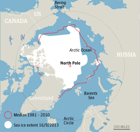 Arctic sea ice extent September 2013. Photograph: guardian.co.uk
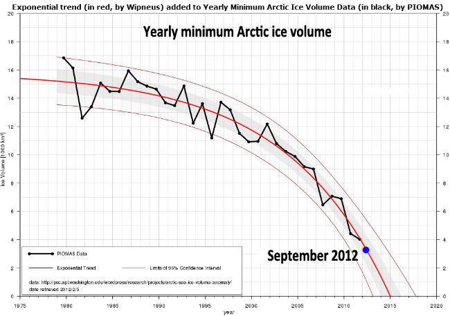
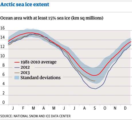 Arctic sea ice extent graph. Photograph: guardian.co.ukThe most dramatic changes have occurred in the past decade. The seven summers with the lowest sea ice minimums were all in the past seven years.

