Confused about the new IPCC’s carbon budget? So am I.

Posted: 17 Oct 2013 12:06 AM PDT

by David Spratt

When the IPCC’s new report on the physical basis of climate change was released in late September, media attention focused on a conclusion from the Summary for Policymakers that the world had emitted just over half of the allowable emissions if global warming is to be kept to 2 degrees Celsius (2°C) of warming.

Unfortunately, because many people think if you have a budget you should spend every last dollar, the “carbon budget” message could be interpreted as saying there is plenty of budget left to spend. The respected climate researcher Ken Caldeira told Climate Progress that the carbon budget concept is dangerous for two reasons:

There are no such things as an “allowable carbon dioxide (CO2) emissions.” There are only “damaging CO2 emissions” or “dangerous CO2 emissions.” Every CO2 emission causes additional damage and creates additional risk. Causing additional damage and creating additional risk with our CO2 emissions should not be allowed.
If you look at how our politicians operate, if you tell them you have a budget of XYZ, they will spend XYZ. Politicians will reason: “If we’re not over budget, what’s to stop us to spending? Let the guys down the road deal with it when the budget has been exceeded.” The CO2 emissions budget framing is a recipe for delaying concrete action now.

And the idea that 2°C of warming is safe is not a sustainable proposition. Prof. Kevin Anderson says that “the impacts associated with 2°C have been revised upwards, sufficiently so that 2°C now more appropriately represents the threshold between ‘dangerous’ and ‘extremely dangerous’ climate change”.

Typical of the media’s coverage of IPCC 2013 was The Guardian’s headline: “IPCC: 30 years to climate calamity if we carry on blowing the carbon budget. Global 2C warming threshold will be breached within 30 years, leading scientists report, with humans unequivocally to blame” and its reporting that:

The scientists found that to hold warming to 2°C, total emissions cannot exceed 1,000 gigatons of carbon. Yet by 2011, more than half of that total “allowance” – 531 gigatons – had already been emitted.

But hold on, I thought the current level of greenhouse gases was enough in the long run to produce 2°C of warming? This is what researchers such as Ramanthan and Feng found back in 2008:

The observed increase in the concentration of greenhouse gases (GHGs) since the pre-industrial era has most likely committed the world to a warming of 2.4°C (1.4°C to 4.3°C) above the preindustrial surface temperatures.

It takes a while for greenhouse gases to produce their full warming effect because 90% of the additional energy goes into heating the oceans and another 7% into melting ice sheets. This is called thermal inertia, and it means that after an increase in the atmospheric greenhouse gas level, about one-third is realised as a temperature increase during the first decade, getting to two-thirds of the warming potential takes 50 years, and most of the rest is realised within a century. So for emissions back in the 1960s, we have felt about two-thirds of the warming; for emissions around 2000, we have felt only one-third of the heating effect so far.

When, after a burst of greenhouse gas emissions, all these processes have worked through the climate system, the resultant effect on temperature is known as equilibrium climate sensitivity (ECS).  This defines the amount of warming for a doubling of greenhouse gas levels, which the new IPCC report finds to be in the range of 1.5–4.5°C, with a median of around 3°C.   From this, we can calculate for the present level of all greenhouse gases of around 478 parts per million carbon dioxide equivalent (ppm CO2e), the equilibrium temperature increase will be 2.3°C if ECS is taken as 3°C.

So how can this be reconciled with the IPCC “headline” story that there are plenty of emissions left in the carbon budget for 2°C of warming?

The new Climate Council’s Prof. Will Steffen says that:

This budget may, in fact, be rather generous. Accounting for non-CO2 greenhouse gases, including the possible release of methane from melting permafrost and ocean sediments, or increasing the probability of meeting the 2°C target all imply a substantially lower carbon budget.

Here’s some pointers as to why.

1. OTHER GREENHOUSE GASES  The budget is for CO2 emissions only, and does not include other greenhouse gases. When these “non-CO2 forcings” are included, the IPCC’s Summary for Policy Makers says the total allowable emissions is 800 gigatonnes of carbon (GtC) for a 66% chance of not exceeding 2°C. Take away the 530 GtC already omitted, and the budget remaining is now 270 GtC.  That a lot less than the “half of 1000 GtC” line that led the news.

2. RISK  And what if didn’t want a one-in-three risk of exceeding 2°C?  That would be very prudent given the escalating impacts above 2°C. The IPCC report doesn’t seem to give the answer.  But an earlier report by Anderson and Bows, quoting work by Meinshausen, said that:

to provide a 93 per cent mid-value probability of not exceeding 2°C, the concentration would need to be stabilized at, or below, 350 ppmv CO2e, i.e. below current levels.

In other words, if you want a very low risk of not exceeding 2°C, there is probably no budget left.   Let’s hope this figure can be clarified.

3. ARCTIC SEA ICE  The IPCC’s carbon budget relies on Coupled Model Intercomparison Project Phase 5 (CMIP5) computer modelling results. In another part of the report, results are given for the ~2°C warming scenario (known as RCP2.6) of a 43% reduction in September Arctic sea-ice extent by end of 21st century (compared to a 1985–2005 reference period).  This is so at odds with the reality on the ground as to be not credible.  In just 30 years and with warming of less than 1°C, the sea-ice extent has dropped by half, and the sea-ice volume by more than three-quarters.  Switched-on Arctic researchers suggest that the Arctic will be sea-ice free in summer within the next decade or so, as discussed here and here and here.

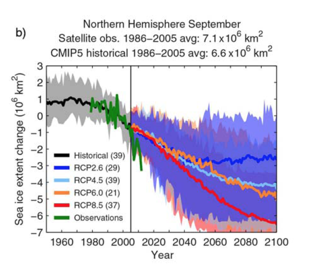Changes in September sea-ice conditions from IPCC for four scenarios using CMIP5, and observations (green line)

In fact the IPCC projection for September sea-ice extent by century’s end (deep blue line on figure at right) for ~2°C of warming is greater than the actual conditions now (green line) with less than 1°C of warming.  Losing the sea-ice earlier than the IPCC projects will change the planet’s surface reflectivity (albedo) and drive further warming. This, again, would reduce the carbon budget for 2°C this century, but in appears this has not been accounted for fully using the CMIP5 Arctic sea-ice results.

4. CARBON STORES The Summary for Policymakers offers this qualification:

A lower warming target, or a higher likelihood of remaining below a specific warming target, will require lower cumulative CO2 emissions. Accounting for warming effects of increases in non-CO2 greenhouse gases, reductions in aerosols, or the release of greenhouse gases from permafrost will also lower the cumulative CO2 emissions for a specific warming target.

In December 2012, the UNEP reported that “the IPCC Fifth Assessment Report, due for release in stages between September 2013 and October 2014, will not include the potential effects of the permafrost carbon feedback on global climate.”  Yet even for the ~2°C warming pathway, permafrost release of greenhouse gases is pertinent. As I reported recently in Is climate change already dangerous?:

A 2012 UNEP report on Policy implications of warming permafrost says the recent observations “indicate that large-scale thawing of permafrost may have already started.”  In February 2013, scientists using radiometric dating techniques on Russian cave formations to measure historic melting rates warned that a +1.5ºC global rise in temperature compared to pre-industrial was enough to start a general permafrost melt.  Vaks, Gutareva et al. found that “global climates only slightly warmer than today are sufficient to thaw extensive regions of permafrost.” Vaks says that: “1.5ºC appears to be something of a tipping point”.

And in April 2011, the paper “Amount and timing of permafrost carbon release in response to climate warming” concluded:

The thaw and release of carbon currently frozen in permafrost will increase atmospheric CO2 concentrations and amplify surface warming to initiate a positive permafrost carbon feedback (PCF) on climate…. [Our] estimate may be low because it does not account for amplified surface warming due to the PCF itself….
We predict that the PCF will change the arctic from a carbon sink to a source after the mid-2020s and is strong enough to cancel 42-88% of the total global land sink. The thaw and decay of permafrost carbon is irreversible and accounting for the PCF will require larger reductions in fossil fuel emissions to reach a target atmospheric CO2 concentration.

For the other three IPCC warming scenarios, permafrost must be a key component. Climate Progress reported in 2012 that:

Back in 2005, before the IPCC’s Fourth Assessment, a major study led by NCAR climate researcher David Lawrence, found that virtually the entire top 11 feet of permafrost around the globe could disappear by the end of this century. Using the first “fully interactive climate system model” applied to study permafrost, the researchers found that if we tried to stabilize CO2 concentrations in the air at 550 ppm, permafrost would plummet from over 4 million square miles today to 1.5 million.
That matters because the permafrost permamelt contains a staggering “1.5 trillion tons of frozen carbon, about twice as much carbon as contained in the atmosphere, much of which would be released as methane.  Methane is 25 times as potent a heat-trapping gas as CO2 over a 100 year time horizon, but 72 to 100 times as potent over 20 years!

All of which suggests to me that for a high probability of not exceeding 2C of warming, and including the likely impacts of a period of sea-ice-free summer conditions in the Arctic sooner rather than later, and significant release of CO2 and methane from Arctic permafrost stores, then the available carbon budget is probably zero, or less.

But that real-world question is not one to which I could find an answer in the IPCC report.

NOT DISCUSSED: At a broader level, the IPCC physical basis report seems weak on many Arctic-related issues.  As far as I can see:

• The predictions of sea-ice loss are so discordant with recent observations as to be not credible.
• Decline in Arctic sea-ice thickness (a more robust indicator than extent) is not discussed.
• While the release of CO2 or methane to the atmosphere from thawing permafrost carbon stocks over the 21st century is assessed,  the other very large sources of Arctic methane (such as sub-sea floor clathrates) are not mentioned.
• The permafrost thaw emissions is only given as carbon, not assessed as methane and as CO2, which have very different radiative forcing impacts.
• The impacts of Arctic-derived carbon cycle positive feedbacks such as permafrost loss on future temperature projections and on allowable carbon budgets are not given.
• No mention is made of the cascading additive effect of multiple Arctic positive feedbacks on the rate of global warming, nor an assessment of Arctic amplification sensitivity.

Sea Level Rise In The 5th IPCC Report

By Stefan Rahmstorf

15 October, 2013
Realclimate.org

What is happening to sea levels? That was perhaps the most controversial issue in the 4th IPCC report of 2007. The new report of the Intergovernmental Panel on Climate Change is out now, and here I will discuss what IPCC has to say about sea-level rise (as I did here after the 4th report).

Let us jump straight in with the following graph which nicely sums up the key findings about past and future sea-level rise: (1) global sea level is rising, (2) this rise has accelerated since pre-industrial times and (3) it will accelerate further in this century. The projections for the future are much higher and more credible than those in the 4th report but possibly still a bit conservative, as we will discuss in more detail below. For high emissions IPCC now predicts a global rise by 52-98 cm by the year 2100, which would threaten the survival of coastal cities and entire island nations. But even with aggressive emissions reductions, a rise by 28-61 cm is predicted. Even under this highly optimistic scenario we might see over half a meter of sea-level rise, with serious impacts on many coastal areas, including coastal erosion and a greatly increased risk of flooding.

Fig. 1. Past and future sea-level rise. For the past, proxy data are shown in light purple and tide gauge data in blue. For the future, the IPCC projections for very high emissions (red, RCP8.5 scenario) and very low emissions (blue, RCP2.6 scenario) are shown. Source: IPCC AR5 Fig. 13.27.

In addition to the global rise IPCC extensively discusses regional differences, as shown for one scenario below. For reasons of brevity I will not discuss these further in this post.

Fig. 2. Map of sea-level changes up to the period 2081-2100 for the RCP4.5 scenario (which one could call late mitigation, with emissions starting to fall globally after 2040 AD). Top panel shows the model mean with 50 cm global rise, the following panels show the low and high end of the uncertainty range for this scenario. Note that even under this moderate climate scenario, the northern US east coast is risking a rise close to a meter, drastically increasing the storm surge hazard to cities like New York. Source: IPCC AR5 Fig. 13.19.

I recommend to everyone with a deeper interest in sea level to read the sea level chapter of the new IPCC report (Chapter 13) – it is the result of a great effort by a group of leading experts and an excellent starting point to understanding the key issues involved. It will be a standard reference for years to come.

Past sea-level rise

Understanding of past sea-level changes has greatly improved since the 4th IPCC report. The IPCC writes:

Proxy and instrumental sea level data indicate a transition in the late 19th to the early 20th century from relatively low mean rates of rise over the previous two millennia to higher rates of rise (high confidence). It is likely that the rate of global mean sea level rise has continued to increase since the early 20th century.

Adding together the observed individual components of sea level rise (thermal expansion of the ocean water, loss of continental ice from ice sheets and mountain glaciers, terrestrial water storage) now is in reasonable agreement with the observed total sea-level rise.

Models are also now able to reproduce global sea-level rise from 1900 AD better than in the 4th report, but still with a tendency to underestimation. The following IPCC graph shows a comparison of observed sea level rise (coloured lines) to modelled rise (black).

Fig. 3. Modelled versus observed global sea-level rise. (a) Sea level relative to 1900 AD and (b) its rate of rise. Source: IPCC AR5 Fig. 13.7.

Taken at face value the models (solid black) still underestimate past rise. To get to the dashed black line, which shows only a small underestimation, several adjustments are needed.

(1) The mountain glacier model is driven by observed rather than modelled climate, so that two different climate histories go into producing the dashed black line: observed climate for glacier melt and modelled climate for ocean thermal expansion.

(2) A steady ongoing ice loss from ice sheets is added in – this has nothing to do with modern warming but is a slow response to earlier climate changes. It is a plausible but highly uncertain contribution – the IPCC calls the value chosen “illustrative” because the true contribution is not known.

(3) The model results are adjusted for having been spun up without volcanic forcing (hard to believe that this is still an issue – six years earlier we already supplied our model results spun up with volcanic forcing to the AR4). Again this is a plausible upward correction but of uncertain magnitude, since the climate response to volcanic eruptions is model-dependent.

The dotted black line after 1990 makes a further adjustment, namely adding in the observed ice sheet loss which as such is not predicted by models. The ice sheet response remains a not yet well-understood part of the sea-level problem, and the IPCC has only “medium confidence” in the current ice sheet models.

One statement that I do not find convincing is the IPCC’s claim that “it is likely that similarly high rates [as during the past two decades] occurred between 1920 and 1950.” I think this claim is not well supported by the evidence. In fact, a statement like “it is likely that recent high rates of SLR are unprecedented since instrumental measurements began” would be more justified.

The lower panel of Fig. 3 (which shows the rates of SLR) shows that based on the Church & White sea-level record, the modern rate measured by satellite altimeter is unprecedented – even the uncertainty ranges of the satellite data and those of the Church & White rate between 1920 and 1950 do not overlap. The modern rate is also unprecedented for the Ray and Douglas data although there is some overlap of the uncertainty ranges (if you consider both ranges). There is a third data set (not shown in the above graph) by Wenzel and Schröter (2010) for which this is also true. The only outlier set which shows high early rates of SLR is the Jevrejeva et al. (2008) data – and this uses a bizarre weighting scheme, as we have discussed here at Realclimate. For example, the Northern Hemisphere ocean is weighted more strongly than the Southern Hemisphere ocean, although the latter has a much greater surface area. With such a weighting movements of water within the ocean, which cannot change global-mean sea level, erroneously look like global sea level changes. As we have shown in Rahmstorf et al. (2012), much or most of the decadal variations in the rate of sea-level rise in tide gauge data are probably not real changes at all, but simply an artefact of inadequate spatial sampling of the tide gauges. (This sampling problem has now been overcome with the advent of satellite data from 1993 onwards.) But even if we had no good reason to distrust decadal variations in the Jevrejeva data and treated all data sets the same, three out of four global tide gauge compilations show recent rates of rise that are unprecedented – enough for a “likely” statement in IPCC terms.

Future sea-level rise

For an unmitigated future rise in emissions (RCP8.5), IPCC now expects between a half metre and a metre of sea-level rise by the end of this century. The best estimate here is 74 cm.

On the low end, the range for the RCP2.6 scenario is 28-61 cm rise by 2100, with a best estimate of 44 cm. Now that is very remarkable, given that this is a scenario with drastic emissions reductions starting in a few years from now, with the world reaching zero emissions by 2070 and after that succeeding in active carbon dioxide removal from the atmosphere. Even so, the expected sea-level rise will be almost three times as large as that experienced over the 20th Century (17 cm). This reflects the large inertia in the sea-level response – it is very difficult to make sea-level rise slow down again once it has been initiated. This inertia is also the reason for the relatively small difference in sea-level rise by 2100 between the highest and lowest emissions scenario (the ranges even overlap) – the major difference will only be seen in the 22nd century.

There has been some confusion about those numbers: some media incorrectly reported a range of only 26-82 cm by 2100, instead of the correct 28-98 cm across all scenarios. I have to say that half of the blame here lies with the IPCC communication strategy. The SPM contains a table with those numbers – but they are not the rise up to 2100, but the rise up to the mean over 2081-2100, from a baseline of the mean over 1985-2005. It is self-evident that this is too clumsy to put in a newspaper or TV report so journalists will say “up to 2100”. So in my view, IPCC would have done better to present the numbers up to 2100 in the table (as we do below), so that after all its efforts to get the numbers right, 16 cm are not suddenly lost in the reporting.

Table 1: Global sea-level rise in cm by the year 2100 as projected by the IPCC AR5. The values are relative to the mean over 1986-2005, so subtract about a centimeter to get numbers relative to the year 2000.

And then of course there are folks like the professional climate change down-player Björn Lomborg, who in an international newspaper commentary wrote that IPCC gives “a total estimate of 40-62 cm by century’s end” – and also fails to mention that the lower part of this range requires the kind of strong emissions reductions that Lomborg is so viciously fighting.

The breakdown into individual components for an intermediate scenario of about half a meter of rise is shown in the following graph.

Fig. 4. Global sea-level projection of IPCC for the RCP6.0 scenario, for the total rise and the individual contributions.

Higher projections than in the past

To those who remember the much-discussed sea-level range of 18-59 cm from the 4th IPCC report, it is clear that the new numbers are far higher, both at the low and the high end. But how much higher they are is not straightforward to compare, given that IPCC now uses different time intervals and different emissions scenarios. But a direct comparison is made possible by table 13.6 of the report, which allows a comparison of old and new projections for the same emissions scenario (the moderate A1B scenario) over the time interval 1990-2100(*). Here the numbers:

AR4: 37 cm (this is the standard case that belongs to the 18-59 cm range).
AR4+suisd: 43 cm (this is the case with “scaled-up ice sheet discharge” – a questionable calculation that was never validated, emphasised or widely reported).
AR5: 60 cm.

We see that the new estimate is about 60% higher than the old standard estimate, and also a lot higher than the AR4 attempt at including rapid ice sheet discharge.

The low estimates of the 4th report were already at the time considered too low by many experts – there were many indications of that (which we discussed back then), including the fact that the process models used by IPCC greatly underestimated the past observed sea-level rise. It was clear that those process models were not mature, and that was the reason for the development of an alternative, semi-empirical approach to estimating future sea-level rise. The semi-empirical models invariably gave much higher future projections, since they were calibrated with the observed past rise.

However, the higher projections of the new IPCC report do not result from including semi-empirical models. Remarkably, they have been obtained by the process models preferred by IPCC. Thus IPCC now confirms with its own methods that the projections of the 4th report were too low, which was my main concern at the time and the motivation for publishing my paper in Science in 2007. With this new generation of process models, the discrepancy to the semi-empirical models has narrowed considerably, but a difference still remains.

Should the semi-empirical models have been included in the uncertainty range of the IPCC projections? A number of colleagues that I have spoken to think so, and at least one has said so in public. The IPCC argues that there is “no consensus” on the semi-empirical models – true, but is this a reason to exclude or include them in the overall uncertainty that we have in the scientific community? I think there is likewise no consensus on the studies that have recently argued for a lower climate sensitivity, yet the IPCC has widened the uncertainty range to encompass them. The New York Times concludes from this that the IPCC is “bending over backward to be scientifically conservative”. And indeed one wonders whether the semi-empirical models would have been also excluded had they resulted in lower estimates of sea-level rise, or whether we see “erring on the side of the least drama” at work here.

What about the upper limit?

Coastal protection professionals require a plausible upper limit for planning purposes, since coastal infrastructure needs to survive also in the worst case situation. A dike that is only “likely” to be good enough is not the kind of safety level that coastal engineers want to provide; they want to be pretty damn certain that a dike will not break. Rightly so.

The range up to 98 cm is the IPCC’s “likely” range, i.e. the risk of exceeding 98 cm is considered to be 17%, and IPCC adds in the SPM that “several tenths of a meter of sea level rise during the 21st century” could be added to this if a collapse of marine-based sectors of the Antarctic ice sheet is initiated. It is thus clear that a meter is not the upper limit.

It is one of the fundamental philosophical problems with IPCC (causing much debate already in conjunction with the 4th report) that it refuses to provide an upper limit for sea-level rise, unlike other assessments (e.g. the sea-level rise scenarios of NOAA (which we discussed here) or the guidelines of the US Army Corps of Engineers). This would be an important part of assessing the risk of climate change, which is the IPCC’s role (**). Anders Levermann (one of the lead authors of the IPCC sea level chapter) describes it thus:

In the latest assessment report of the IPCC we did not provide such an upper limit, but we allow the creative reader to construct it. The likely range of sea level rise in 2100 for the highest climate change scenario is 52 to 98 centimeters (20 to 38 inches.). However, the report notes that should sectors of the marine-based ice sheets of Antarctic collapse, sea level could rise by an additional several tenths of a meter during the 21st century. Thus, looking at the upper value of the likely range, you end up with an estimate for the upper limit between 1.2 meters and, say, 1.5 meters. That is the upper limit of global mean sea-level that coastal protection might need for the coming century.

Outlook

For the past six years since publication of the AR4, the UN global climate negotiations were conducted on the basis that even without serious mitigation policies global sea-level would rise only between 18 and 59 cm, with perhaps 10 or 20 cm more due to ice dynamics. Now they are being told that the best estimate for unmitigated emissions is 74 cm, and even with the most stringent mitigation efforts, sea level rise could exceed 60 cm by the end of century. It is basically too late to implement measures that would very likely prevent half a meter rise in sea level. Early mitigation is the key to avoiding higher sea level rise, given the slow response time of sea level (Schaeffer et al. 2012). This is where the “conservative” estimates of IPCC, seen by some as a virtue, have lulled policy makers into a false sense of security, with the price having to be paid later by those living in vulnerable coastal areas.

Is the IPCC AR5 now the final word on process-based sea-level modelling? I don’t think so. I see several reasons that suggest that process models are still not fully mature, and that in future they might continue to evolve towards higher sea-level projections.

1. Although with some good will one can say the process models are now consistent with the past observed sea-level rise (the error margins overlap), the process models remain somewhat at the low end in comparison to observational data.

2. Efforts to model sea-level changes in Earth history tend to show an underestimation of past sea-level changes. E.g., the sea-level high stand in the Pliocene is not captured by current ice sheet models. Evidence shows that even the East Antarctic Ice Sheet – which is very stable in models – lost significant amounts of ice in the Pliocene.

3. Some of the most recent ice sheet modelling efforts that I have seen discussed at conferences – the kind of results that came too late for inclusion in the IPCC report – point to the possibility of larger sea-level rise in future. We should keep an eye out for the upcoming scientific papers on this.

4. Greenland might melt faster than current models capture, due to the “dark snow” effect. Jason Box, a glaciologist who studies this issue, has said:

There was controversy after AR4 that sea level rise estimates were too low. Now, we have the same problem for AR5 [that they are still too low].

Thus, I would not be surprised if the process-based models will have closed in further on the semi-empirical models by the time the next IPCC report gets published. But whether this is true or not: in any case sea-level rise is going to be a very serious problem for the future, made worse by every ton of CO2 that we emit. And it is not going to stop in the year 2100 either. By 2300, for unmitigated emissions IPCC projects between 1 and more than 3 meters of rise.

Weblink

I’m usually suspicious of articles that promise to look “behind the scenes”, but this one by Paul Voosen is not sensationalist but gives a realistic and matter-of-fact insight into the inner workings of the IPCC, for the sea-level chapter. Recommended reading!

—
(*) Note: For the AR5 models table 13.6 gives 58 cm from 1996; we made that 60 cm from 1990.

(**) The Principles Governing IPCC Work explicitly state that its role is to “assess…risk”, albeit phrased in a rather convoluted sentence:

The role of the IPCC is to assess on a comprehensive, objective, open and transparent basis the scientific, technical and socio-economic information relevant to understanding the scientific basis of risk of human-induced climate change, its potential impacts and options for adaptation and mitigation.

References

1. J.A. Church, and N.J. White, “Sea-Level Rise from the Late 19th to the Early 21st Century”, Surveys in Geophysics, vol. 32, pp. 585-602, 2011. http://dx.doi.org/10.1007/s10712-011-9119-1

2. R.D. Ray, and B.C. Douglas, “Experiments in reconstructing twentieth-century sea levels”, Progress in Oceanography, vol. 91, pp. 496-515, 2011. http://dx.doi.org/10.1016/j.pocean.2011.07.021

3. M. Wenzel, and J. Schröter, “Reconstruction of regional mean sea level anomalies from tide gauges using neural networks”, Journal of Geophysical Research, vol. 115, 2010. http://dx.doi.org/10.1029/2009JC005630

4. S. Jevrejeva, J.C. Moore, A. Grinsted, and P.L. Woodworth, “Recent global sea level acceleration started over 200 years ago?”, Geophysical Research Letters, vol. 35, 2008. http://dx.doi.org/10.1029/2008GL033611

5. S. Rahmstorf, M. Perrette, and M. Vermeer, “Testing the robustness of semi-empirical sea level projections”, Climate Dynamics, vol. 39, pp. 861-875, 2012. http://dx.doi.org/10.1007/s00382-011-1226-7

6. S. Rahmstorf, “A Semi-Empirical Approach to Projecting Future Sea-Level Rise”, Science, vol. 315, pp. 368-370, 2007. http://dx.doi.org/10.1126/science.1135456

7. M. Schaeffer, W. Hare, S. Rahmstorf, and M. Vermeer, “Long-term sea-level rise implied by 1.5 °C and 2 °C warming levels”, Nature Climate Change, vol. 2, pp. 867-870, 2012. http://dx.doi.org/10.1038/nclimate1584

Stefan Rahmstorf: A physicist and oceanographer by training, Stefan Rahmstorf has moved from early work in general relativity theory to working on climate issues. He has done research at the New Zealand Oceanographic Institute, at the Institute of Marine Science in Kiel and since 1996 at the Potsdam Institute for Climate Impact Research in Germany (in Potsdam near Berlin). His work focuses on the role of ocean currents in climate change, past and present. In 1999 Rahmstorf was awarded the $ 1 million Centennial Fellowship Award of the US-based James S. McDonnell foundation. Since 2000 he teaches physics of the oceans as a professor at Potsdam University. Rahmstorf is a member of the Advisory Council on Global Change of the German government and of the Academia Europaea. He is a lead author of the paleoclimate chapter of the 4th assessment report of the

“Very Generous Immigration Program” Pushing Out Would Be Home Buyers

Charlie Wood – 350.org Australia <charlie@350.org>	6:43 PM (11 minutes ago)
to me

Images are not displayed. Display images below – Always display images from charlie@350.org

350.org is building a global movement to solve the climate crisis. Connect with us on Facebook and Twitter, and sign up for email alerts. You can help power our work by getting involved locally, sharing your story, and donating here. To change your email address or update your contact info, click here.