Solar Parabolic trough

Parabolic trough

A parabolic trough consists of a linear parabolic reflector that concentrates light onto a receiver positioned along the reflector’s focal line. The receiver is a tube positioned directly above the middle of the parabolic mirror and filled with a working fluid. The reflector follows the sun during the daylight hours by tracking along a single axis. A working fluid (e.g.molten salt^[13]) is heated to 150–350 °C (423–623 K (302–662 °F)) as it flows through the receiver and is then used as a heat source for a power generation system.^[14] Trough systems are the most developed CSP technology. The Solar Energy Generating Systems (SEGS) plants in California, the world’s first commercial parabolic trough plants, Acciona’s Nevada Solar One near Boulder City, Nevada, and Andasol, Europe’s first commercial parabolic trough plant are representative, alongside with Plataforma Solar de Almería‘s SSPS-DCS test facilities in Spain.^[15]

[edit]Fresnel reflectors

Liddell Power Station‘s Compact Linear Fresnel reflectors are not as efficient as parabolic mirrors but are much cheaper.

Main article:Compact Linear Fresnel Reflector

Fresnel reflectors are made of many thin, flat mirror strips to concentrate sunlight onto tubes through which working fluid is pumped. Flat mirrors allow more reflective surface in the same amount of space as a parabolic reflector, thus capturing more of the available sunlight, and they are much cheaper than parabolic reflectors. Fresnel reflectors can be used in various size CSPs.^[16]^[17]

[edit]Dish Stirling

Main article: Dish Stirling

A dish Stirling or dish engine system consists of a stand-aloneparabolic reflector that concentrates light onto a receiver positioned at the reflector’s focal point. The reflector tracks the Sun along two axes. The working fluid in the receiver is heated to 250–700 °C (523–973 K (482–1292 °F)) and then used by aStirling engine to generate power.^[14] Parabolic-dish systems provide the highest solar-to-electric efficiency among CSP technologies, and their modular nature provides scalability. TheStirling Energy Systems (SES) and Science Applications International Corporation (SAIC) dishes at UNLV, andAustralian National University‘s Big Dish in Canberra, Australia are representative of this technology.

[edit]Solar power tower

Main article: Solar power tower

A solar power tower consists of an array of dual-axis tracking reflectors (heliostats) that concentrate sunlight on a central receiver atop a tower; the receiver contains a fluid deposit, which can consist of sea water. The working fluid in the receiver is heated to 500–1000 °C (773–1273 K (932–1832 °F)) and then used as a heat source for a power generation or energy storage system.^[14] Power-tower development is less advanced than trough systems, but they offer higher efficiency and better energy storage capability. The Solar Two in Daggett, California and the CESA-1 in Plataforma Solar de Almeria Almeria, Spain, are the most representative demonstration plants. The Planta Solar 10 (PS10) in Sanlucar la Mayor, Spain is the first commercial utility-scale solar power tower in the world. eSolar‘s 5 MW Sierra SunTower, located in Lancaster, California, is the only CSP tower facility operating in North America.

[edit]Deployment around the world

The commercial deployment of CSP plants started by 1984 in the US with the SEGS plants until 1990 when the last SEGS plant was completed. Since 1990 to 2007 there were no more CSP plants built in the world.

Year	1984	1985	1989	1990	2006	2007	2008	2009	2010	2011	2012*
CSP power (MW)	14	60	200	80	1	74	55	178.50	306.50	625	180
ISCC power (MW)	–	–	–	–	–	–	–	–	22	97	40
Total (cumulative) (MW)	14	74	274	354	355	429	484	622.50	991	1713	2183

Figures for 2012 are as of July. ^[18]

[edit]Efficiency

For thermodynamic solar systems, the maximum solar-to-work (ex: electricity) efficiency $eta$ can be deduced by considering boththermal radiation properties and Carnot’s principle.^[19] Indeed, solar irradiation must first be converted into heat via a solar receiver with an efficiency $eta_{Receiver}$ ; then this heat is converted into work with Carnot efficiency $eta_{Carnot}$ . Hence, for a solar receiver providing a heat source at temperature T_Hand a heat sink at temperature T° (e.g.: atmosphere at T° = 300 K) :

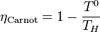
$eta = eta_mathrm{Receiver} cdot eta_mathrm{Carnot}$

with $eta_mathrm{Carnot} = 1 - frac{T^0}{T_H}$

and $eta_mathrm{Receiver} = frac{Q_mathrm{absorbed}-Q_mathrm{lost}}{Q_mathrm{solar}}$

where $Q_mathrm{solar}$ , $Q_mathrm{absorbed}$ , $Q_mathrm{lost}$ are respectively the incoming solar flux and the fluxes absorbed and lost by the system solar receiver.

For a solar flux I (e.g. I = 1000 W/m²) concentrated C times with an efficiency $eta_{Optics}$ on the system solar receiver with a collecting area A and an absorptivity $alpha$ :

$Q_mathrm{solar} = eta_mathrm{Optics} I C A$ ,

$Q_mathrm{absorbed} = alpha Q_mathrm{solar}$ ,

For simplicity’s sake, one can assume that the losses are only radiative ones (a fair assumption for high temperatures), thus for a reradiating area A and an emissivity $epsilon$ applying the Stefan-Boltzmann law yields:

$Q_mathrm{lost} = A epsilon sigma T_H^4$

Simplifying these equations by considering perfect optics ( $eta_mathrm{Optics}$ = 1), collecting and reradiating areas equal and maximum absorptivity and emissivity ( $alpha$ = 1, $epsilon$ = 1) then substituting in the first equation gives

$eta = left(1 - frac {sigma T_H^4 }{IC} right) cdot left( 1 - frac{T^0}{T_H} right)$

One sees that efficiency does not simply increase monotonically with the receiver temperature. Indeed, the higher the temperature, the higher the Carnot efficiency, but also the lower the receiver efficiency. Hence, the maximum reachable temperature (i.e.: when the receiver efficiency is null, blue curve on the figure below) is: $T_mathrm{max} = left({frac {IC}{sigma}} right)^{0.25}$

There is a temperature T_opt for which the efficiency is maximum, i.e. when the efficiency derivative relative to the receiver temperature is null:

$frac{deta}{dT_H}(T_mathrm{opt}) = 0$

Consequently, this lead us to the following equation:

$T_{opt}^5-(0.75T^0)T_mathrm{opt}^4-frac{T^0IC}{4sigma} = 0$

Solving numerically this equation allows to obtain the optimum process temperature according to the solar concentration ratioC (red curve on the figure below)

C	500	1000	5000	10000	45000 (max. for Earth)
T_max	1720	2050	3060	3640	5300
T_opt	970	1100	1500	1720	2310

[edit]Costs

As of 9 September 2009, the cost of building a CSP station was typically about US$2.50 to $4 per watt,^[20] while the fuel (the sun’s radiation) is free. Thus a 250 MW CSP station would have cost $600–1000 million to build. That works out to $0.12 to $0.18/kwh.^[20]. New CSP stations may be economically competitive with fossil fuels. Nathaniel Bullard, a solar analyst at Bloomberg New Energy Finance, has calculated that the cost of electricity at the Ivanpah Solar Power Facility, a project under construction in Southern California, will be lower than that from photovoltaic power and about the same as that from natural gas.^[21] However, in November 2011, Google announced that they would not invest further in CSP projects due to the rapid price decline of photovoltaics. Google spent $168 million on BrightSource.^[22]^[23] IRENA has published on June 2012 a series of studies titled: “Renewable Energy Cost Analysis”. The CSP study shows the cost of both building and operation of CSP plants. Costs are expected to decrease, but there are insufficient installations to clearly establish the learning curve. As of March 2012, there were 1.9 GW of CSP installed, with 1.8 GW of that being parabolic trough.^[24]